Estimating Dry Weight of Composition Material

While trying to remelt some old composition rollers recently, I found that some of the material wouldn’t melt. Neither higher temperatures nor additional water helped. All I ended up with was a lumpy soup, from which I strained the lumps and let the liquid portion set in a measuring cup.

I was curious as to how much of the original 250g of composition material I has managed to recover, but the sample in the cup contained quite a bit of extra water.

I had two choices: let the sample air dry until it no longer lost any weight, or sample the weight through a period of consistent drying conditions and use the changing weight to estimate the final dry weight.

The second method might require less time so I decided to try it. I cut off a about quarter of the hardened composition material and placed it on a piece of aluminum foil on the pan of my precision scale, which has a resolution of 100μg. The scale has a glass enclosure which I hoped would provide a consistent drying rate.

(warning: Math ahead!)

Drying is a diffusion process: the water must diffuse through to the surface of the material, transfer to the air, and the moisture in the air must diffuse into the atmosphere at large. In such processes, the rate of transfer between two regions depends on the difference in moisture content between them. The result is that the weight of a sample will approach its equilibrium value according to a formula:

$m\left(t\right)=m_{\mathrm{eq}}+(m_{\mathrm{s}}-m_{\mathrm{eq}})e^{-R(t-t_{\mathrm{s}})}$

where $m\left(t\right)$ is the sample mass as a function of time, and $m_{\mathrm{s}}$ is the mass measured at some sampling time $t_{\mathrm{s}}$. The rate of drying is represented by $R$ and $m_{\mathrm{eq}}$ is the ultimate equilibrium mass.

By making measurements of the weight over time this would give several sample points for $m\left(t\right)$, any of which being used to provide $m_{\mathrm{s}}$ and $t_{\mathrm{s}}$. Using this set of sample points, values for $R$ and $m_{\mathrm{eq}}$ could be estimated, with the latter being the ultimate dry weight of the sample.

I did not have any way of fitting the equation of this form to samples, so I transformed the samples and equations into a linear problem, first by taking the time derivative of the function, and using the differences between consecutive samples to approximate the rate of drying at the middle of the time interval:

$\frac{dm}{dt}=-R(m_{\mathrm{s}}-m_{\mathrm{eq}})e^{-R(t-t_{\mathrm{s}})}$

fitted to values $\frac{m_i-m_{i-1}}{t_i-t_{i-1}}$ at time $\frac{t_i+t_{i-1}}{2}$ for pairs of consecutive samples.

To complete the linearization, the logarithm of both the rate samples and $-\frac{dm}{dt}$ is taken. Although the algebra doesn’t care, $m\left(t\right)$ is decreasing with time and so $\frac{dm}{dt}$ is negative and the logarithm of $\frac{m_i-m_{i-1}}{t_i-t_{i-1}}$ will be a complex number which is not easy to graph. Taking the logarithm of the negated value keeps the calculations in real numbers.

$ln(-\frac{dm}{dt})=[ln(R(m_{\mathrm{s}}-m_{\mathrm{eq}}))+R{t}_{\mathrm{s}}]-Rt$

Note that the value in square brackets is a constant. By obtaining parameters $A$ and $B$ for a linear fit to the data in the form

$ln(-\frac{dm}{dt})=At+B$

we see that

$R=-A$

and

$m_{\mathrm{eq}}=m_{\mathrm{s}}-\frac{e^{B-R{t}_{\mathrm{s}}}}{R}=m_{\mathrm{s}}+\frac{e^{B+A{t}_{\mathrm{s}}}}{A}$

Substituting these values back into the original definition of $m\left(t\right)$ yields the formula in terms of the linear fit parameters $A$ and B:

$m\left(t\right)=m_{\mathrm{s}}+\frac{e^{B+A{t}_{\mathrm{s}}}}{A}-\frac{e^B}{A}{e}^{At}$

The sum of the first two terms is equal to $m_{\mathrm{eq}}$ and the last is independent of which sampling is used for $m_{\mathrm{s}}$ and $t_{\mathrm{s}}$. The choice of which sample(s) are used to determine $m_{\mathrm{eq}}$ is somewhat arbitrary. In this analysis I chose to take the mean value $\overline{m_{\mathrm{eq}}}$ calculated from all the samples. A better way might be to weight the later samples more heavily as they are closer to the ultimate equilibrium state.

I measured the sample weight more or less daily over several weeks to see how well this method worked. Here is a chart of $\ln \frac{m_i-m_{i-1}}{t_i-t_{i-1}}$ as a function of $\frac{t_i+t_{i-1}}{2}$ along with a fitted linear function.

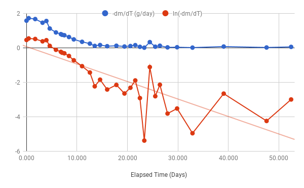
Note that as the sample dries, the day-to-day weight change gets smaller so factors like error in the weigh scale and drying rate variations start to dominate the measured values, causing the charted values to become wilder as time progresses. In particular, the linear function would be a closer fit (with a steeper slope) without the last 3 samples.

The coefficients for the linear fit equation are:

$A$ = -0.102 and $B$ = 0.1

This implies that

$R$ = 0.102 and $\overline{m_{\mathrm{eq}}}$ = 20.73g

These values were plugged back into the original formula for $m\left(t\right)$ and charted against the actual measured values:

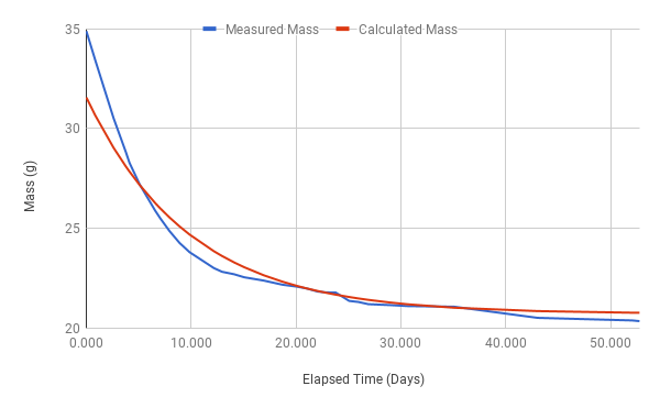Because of the even weighting used to calculate $\overline{m_{\mathrm{eq}}}$ the somewhat absurd effect can be seen that the predicted ultimate weight of 20.73g is greater than actual measured weights from later samples (the last sample weight was 20.36g, and at the time of writing this article, the weight was 19.71g at day 81).

The slower drop of the calculated value in the first 20 days is the result of using the last three “wild” samples in the linear fit model, as discussed above. By taking a linear fit ignoring the last 3 samples, the results are $A$ = -.1525, $B$ = 0.7, and $\overline{m_{\mathrm{eq}}}$ = 21.13g (averaged including the last 3 samples). This gives a much closer fit between calculated and actual weights up to day 35, but $\overline{m_{\mathrm{eq}}}$ is even higher than the actual ultimate weight. These discrepancies are most likely due to the assumption of a single stable equilibrium weight, while in actuality we have progressed from early fall to early winter, resulting in decreasing air humidity, and so $m_{\mathrm{eq}}$ has been a moving target.

Weight vs. Mass

In this analysis I appear to use “weight” and “mass” almost interchangeably. My scale measures weight, but the formulas and analysis work with mass, and I tried to keep the wording correct to reflect this. In practice, the factor relating weight and mass is the earth’s gravity, which is not considered to vary substantially from week to week, and although the scale measures weight, it reads in mass units assuming a standard value for gravity.

Writing this post: MathML vs. WordPress

HTML (the descriptive language for Web pages) includes extensions for displaying equations and such constructs, called MathML. Unfortunately, WordPress, which is the basis for this blog, just can’t seem to leave unrecognized HTML alone and strips it out. As a result I can’t just write the MathML in raw form using the text-mode WP editor because it all vanishes.

Instead I’ve added a plugin, called “WordPress HTML”, which allows pristine literal HTML to be included in posts, but at the expense of having to define these literal bits as named objects, out of line from where they’re used, giving them a (hopefully) meaningful name, and referencing that name with somewhat clunky syntax in the main text of the post. Even ignoring the fact that writing raw MathML is somewhat painful to do, having to name things and place them out-of-line doesn’t help matters in the least!

The only plus to this is that the MathML for something like $\frac{dm}{dt}$ only occurs once no matter how many times I mention $\frac{dm}{dt}$ in the main article text. But even at that, it cannot be referenced in other math definitions, so for instance $-\frac{dm}{dt}$ includes a copy of the definition of $\frac{dm}{dt}$.

Note that this post was updated October 2023 to account for the deprecated <mfenced> no longer being implemented in at least some web browsers, which caused important parentheses to disappear from the visible content.